Factor Analysis of Spectrograms with erpPCA

This tutorial demonstrates how to decompose a grid ECoG spectrogram into spatio-spectral factors using varimax-rotated PCA (erpPCA).

Setup

Python 3.10+ required. Install cogpy with the extras this notebook needs (interactive plots + spectral backend + Jupyter kernel):

pip install "ecogpy[viz,signal,notebook]"

Or install everything at once: pip install "ecogpy[all]". For a development install see Installation.

Note

This is a method demo using a short bundled sample recording. The sample data is not chosen to highlight any particular oscillatory phenomenon. For real analyses (e.g. spindle detection in NREM sleep), use a domain-appropriate recording.

The pipeline is:

1. Load a grid ECoG signal

2. Compute a multitaper spectrogram

3. Build a design matrix (log-power, mean-centred)

4. Fit erpPCA → extract loadings and scores

5. Inspect loadings (which spatial pattern at which frequency)

6. Process factor scores (smooth, threshold, detect events)

Each factor captures a recurring spatio-spectral pattern.

Tip

Why varimax? Rohe & Zeng (2023) show that varimax-rotated PCA is, under mild conditions, equivalent to ICA: when the latent factors are non-Gaussian (leptokurtic, κ > 3), varimax recovers statistically identifiable independent components — the same goal ICA pursues, but via the classical eigendecomposition + rotation route rather than higher-order tensor methods. This makes erpPCA both computationally simple and theoretically grounded.

K. Rohe and M. Zeng, “Vintage factor analysis with Varimax performs statistical inference,” J. R. Stat. Soc. B, vol. 85, no. 4, pp. 1037–1060, 2023. DOI: 10.1093/jrsssb/qkad029

import numpy as np
import xarray as xr
import matplotlib.pyplot as plt
import holoviews as hv

hv.extension("bokeh")

1. Load sample data

load_sample() returns a preprocessed grid ECoG signal with dims (AP, ML, time) at 125 Hz.

from cogpy.datasets import load_sample

sig = load_sample()
print(sig)

<xarray.DataArray 'signal' (AP: 16, ML: 16, time: 932)> Size: 2MB
dask.array<transpose, shape=(16, 16, 932), dtype=float64, chunksize=(16, 16, 932), chunktype=numpy.ndarray>
Coordinates:
  * AP       (AP) int64 128B 0 1 2 3 4 5 6 7 8 9 10 11 12 13 14 15
  * ML       (ML) int64 128B 0 1 2 3 4 5 6 7 8 9 10 11 12 13 14 15
  * time     (time) float64 7kB 0.0 0.008 0.016 0.024 ... 7.424 7.432 7.44 7.448
Attributes:
    fs:       125.0

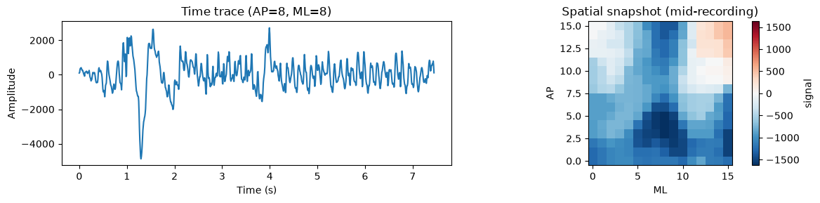
Quick look — single-channel time trace and a spatial snapshot:

fig, axes = plt.subplots(1, 2, figsize=(12, 3))

# Time trace at center electrode
sig.sel(AP=8, ML=8).plot(ax=axes[0])
axes[0].set(title="Time trace (AP=8, ML=8)", xlabel="Time (s)", ylabel="Amplitude")

# Spatial snapshot at one time point
sig.isel(time=sig.sizes["time"] // 2).plot(ax=axes[1], cmap="RdBu_r")
axes[1].set(title="Spatial snapshot (mid-recording)", aspect="equal")
plt.tight_layout()

2. Compute multitaper spectrogram

We use spectrogramx (ghostipy backend) to compute a time-frequency representation for every electrode in the grid.

Three practical considerations for the PCA step:

• Frequency range: clip to frequencies of interest (1–50 Hz) to avoid inflating the variable count.

• Frequency coarsening: average adjacent frequency bins to reduce dimensionality while preserving spectral structure. This is the single most effective knob for controlling runtime.

• Grid subsampling: for large grids, subsample spatially to keep the covariance matrix tractable.

The PCA variable count is n_AP × n_ML × n_freq. The covariance matrix is (n_vars × n_vars), so keeping this under ~3000 is recommended for interactive use.

Note

This tutorial uses aggressive subsampling (8×8 grid, 12 freq bins → 768 variables) to keep the docs build fast (~45 s). For real analyses you can use the full 16×16 grid with 10–25 frequency bins. See Computational considerations at the end.

from cogpy.spectral.specx import spectrogramx

spec = spectrogramx(sig, bandwidth=4.0, nperseg=64, noverlap=56)
spec = spec.compute() if hasattr(spec.data, "compute") else spec

# Clip frequency range and subsample grid
spec = spec.sel(freq=slice(1, 50))
spec = spec.isel(AP=slice(None, None, 2), ML=slice(None, None, 2))  # 8×8

# Coarsen frequency: average pairs of adjacent bins → ~12 bins
# This is the key step for keeping the eigendecomposition fast.
spec = spec.coarsen(freq=2, boundary="trim").mean()

n_vars = spec.sizes["AP"] * spec.sizes["ML"] * spec.sizes["freq"]
print(f"Spectrogram: {spec.shape}")
print(f"PCA variables: {spec.sizes['AP']}×{spec.sizes['ML']}×{spec.sizes['freq']} = {n_vars}")

Spectrogram: (8, 8, 12, 109)
PCA variables: 8×8×12 = 768

Spectrogram at one electrode and mean spectrum across the grid:

mid_ap = spec.AP.values[len(spec.AP) // 2]
mid_ml = spec.ML.values[len(spec.ML) // 2]

spec_img = hv.Image(
    spec.sel(AP=mid_ap, ML=mid_ml),
    kdims=["time", "freq"],
    label="Spectrogram",
).opts(cmap="viridis", colorbar=True, width=500, height=250,
       title=f"Spectrogram at AP={mid_ap}, ML={mid_ml}")

mean_spec = spec.mean(dim=("AP", "ML", "time"))
mean_curve = hv.Curve(
    (mean_spec.freq.values, mean_spec.values),
    kdims=["Frequency (Hz)"], vdims=["Power"],
    label="Mean spectrum",
).opts(width=350, height=250, title="Mean power spectrum", logy=True)

spec_img + mean_curve

3. Build the design matrix

erpPCA operates on a 2D matrix (time, variables). We:

1. Rename dims to SpatSpecDecomposition convention (AP→h, ML→w)

2. Flatten spatial + frequency dims into one axis

3. Log-transform power (stabilises variance)

4. Mean-centre each variable across time

We deliberately avoid z-scoring (dividing by std) here: that would equalise the variance of every channel×frequency variable, giving noise-dominated variables the same weight as signal-rich ones in the covariance matrix.

from cogpy.decomposition.spatspec import SpatSpecDecomposition

mtx = spec.rename({"AP": "h", "ML": "w"})
ss = SpatSpecDecomposition(mtx)

X = ss.designmat(mtx, log=True)
Xc = X - X.mean("time")
Xc.data = np.nan_to_num(Xc.data)

print(f"Design matrix: {Xc.shape[0]} time points × {Xc.shape[1]} variables")

Design matrix: 109 time points × 768 variables

Visualise the design matrix as a heatmap — each row is a time window, each column a (channel, frequency) variable:

hv.Image(
    Xc.data,
    kdims=["Variable", "Time"],
    bounds=(0, 0, Xc.shape[1], Xc.shape[0]),
).opts(
    cmap="RdBu_r", colorbar=True, width=600, height=250,
    title="Design matrix (mean-centred log-power)",
    xlabel="Variable index (h × w × freq)", ylabel="Time window",
    invert_yaxis=True,
)

4. Fit erpPCA

The erpPCA estimator follows the scikit-learn API:

1. Covariance matrix of the design matrix

2. Eigendecomposition

3. Varimax rotation to maximise simple structure

4. Sort factors by explained variance

from cogpy.decomposition.pca import erpPCA

nfac = 8
erp = erpPCA(nfac=nfac, verbose=False)
erp.fit(Xc.data)

print(f"Loadings:   {erp.LR.shape}  (vars × factors)")
print(f"Scores:     {erp.FSr.shape}  (time × factors)")
print(f"Var explained (rotated): {erp.VT[3][:nfac].sum():.1f}%")

computing covariance matrix ...
eigendecomposition ...
Varimax ...

/home/runner/work/cogpy/cogpy/src/cogpy/decomposition/pca.py:275: RuntimeWarning: invalid value encountered in sqrt
  LU = EM * np.sqrt(EV)

Loadings:   (768, 8)  (vars × factors)
Scores:     (109, 8)  (time × factors)
Var explained (rotated): 74.2%

Tip

Short recordings and rank-deficient covariance. When the number of time windows is smaller than the number of variables (as in this demo), the empirical covariance matrix is rank-deficient and the top eigenvalues are over-estimated. A shrinkage covariance estimator (e.g. Ledoit-Wolf) regularises the estimate by pulling eigenvalues toward their grand mean:

from sklearn.covariance import LedoitWolf

erp = erpPCA(nfac=nfac, cov_estimator=LedoitWolf(), verbose=False)
erp.fit(Xc.data)

This is recommended whenever n_time_windows < n_variables.

Variance explained per factor:

var_pct = erp.VT[3][:nfac]
hv.Bars(
    [(f"F{i}", v) for i, v in enumerate(var_pct)],
    kdims=["Factor"], vdims=["Variance (%)"],
).opts(
    width=400, height=250, color="steelblue",
    title="Variance explained per factor (rotated)",
)

5. Reshape into loadings and scores

Reshape the flat loading matrix back into (factor, h, w, freq) and wrap scores as (time, factor) DataArrays.

ss.ldx_set(erp.LR)
ss.ldx_process()
scx = ss.scx_from_FSr(erp.FSr, Xc.time.values)

print(f"Loadings: {ss.ldx.shape}")
print(f"Scores:   {scx.shape}")
print(f"\nFactor summary:")
print(ss.ldx_df[["AP", "ML", "freqmax", "norm"]])

Loadings: (8, 8, 8, 12)
Scores:   (109, 8)

Factor summary:
        AP  ML    freqmax      norm
factor                             
0        0   6   2.929688  4.749759
1       12   0  26.367188  3.766792
2        0   6  22.460938  2.854257
3        2  14  30.273438  2.579805
4       12  12  41.992188  1.994911
5        2   6   6.835938  1.767517
6        8   4  34.179688  1.493770
7       14   0  30.273438  1.479226

/opt/hostedtoolcache/Python/3.11.15/x64/lib/python3.11/site-packages/xarray/core/dataarray.py:6439: FutureWarning: Behaviour of argmin/argmax with neither dim nor axis argument will change to return a dict of indices of each dimension. To get a single, flat index, please use np.argmin(da.data) or np.argmax(da.data) instead of da.argmin() or da.argmax().
  result = self.variable.argmax(dim, axis, keep_attrs, skipna)
/opt/hostedtoolcache/Python/3.11.15/x64/lib/python3.11/site-packages/xarray/core/dataarray.py:6439: FutureWarning: Behaviour of argmin/argmax with neither dim nor axis argument will change to return a dict of indices of each dimension. To get a single, flat index, please use np.argmin(da.data) or np.argmax(da.data) instead of da.argmin() or da.argmax().
  result = self.variable.argmax(dim, axis, keep_attrs, skipna)
/opt/hostedtoolcache/Python/3.11.15/x64/lib/python3.11/site-packages/xarray/core/dataarray.py:6439: FutureWarning: Behaviour of argmin/argmax with neither dim nor axis argument will change to return a dict of indices of each dimension. To get a single, flat index, please use np.argmin(da.data) or np.argmax(da.data) instead of da.argmin() or da.argmax().
  result = self.variable.argmax(dim, axis, keep_attrs, skipna)
/opt/hostedtoolcache/Python/3.11.15/x64/lib/python3.11/site-packages/xarray/core/dataarray.py:6439: FutureWarning: Behaviour of argmin/argmax with neither dim nor axis argument will change to return a dict of indices of each dimension. To get a single, flat index, please use np.argmin(da.data) or np.argmax(da.data) instead of da.argmin() or da.argmax().
  result = self.variable.argmax(dim, axis, keep_attrs, skipna)
/opt/hostedtoolcache/Python/3.11.15/x64/lib/python3.11/site-packages/xarray/core/dataarray.py:6439: FutureWarning: Behaviour of argmin/argmax with neither dim nor axis argument will change to return a dict of indices of each dimension. To get a single, flat index, please use np.argmin(da.data) or np.argmax(da.data) instead of da.argmin() or da.argmax().
  result = self.variable.argmax(dim, axis, keep_attrs, skipna)
/opt/hostedtoolcache/Python/3.11.15/x64/lib/python3.11/site-packages/xarray/core/dataarray.py:6439: FutureWarning: Behaviour of argmin/argmax with neither dim nor axis argument will change to return a dict of indices of each dimension. To get a single, flat index, please use np.argmin(da.data) or np.argmax(da.data) instead of da.argmin() or da.argmax().
  result = self.variable.argmax(dim, axis, keep_attrs, skipna)
/opt/hostedtoolcache/Python/3.11.15/x64/lib/python3.11/site-packages/xarray/core/dataarray.py:6439: FutureWarning: Behaviour of argmin/argmax with neither dim nor axis argument will change to return a dict of indices of each dimension. To get a single, flat index, please use np.argmin(da.data) or np.argmax(da.data) instead of da.argmin() or da.argmax().
  result = self.variable.argmax(dim, axis, keep_attrs, skipna)
/opt/hostedtoolcache/Python/3.11.15/x64/lib/python3.11/site-packages/xarray/core/dataarray.py:6439: FutureWarning: Behaviour of argmin/argmax with neither dim nor axis argument will change to return a dict of indices of each dimension. To get a single, flat index, please use np.argmin(da.data) or np.argmax(da.data) instead of da.argmin() or da.argmax().
  result = self.variable.argmax(dim, axis, keep_attrs, skipna)
/home/runner/work/cogpy/cogpy/src/cogpy/decomposition/spatspec.py:251: FutureWarning: In a future version of xarray the default value for coords will change from coords='different' to coords='minimal'. This is likely to lead to different results when multiple datasets have matching variables with overlapping values. To opt in to new defaults and get rid of these warnings now use `set_options(use_new_combine_kwarg_defaults=True) or set coords explicitly.
  ldx_slc_maxfreq = xr.concat(spat_ldx_list, "factor")

6. Visualise loadings

Spatial maps (HoloViews)

Each factor’s spatial map at its peak frequency, laid out in a grid. The × marks the peak electrode. These are static HoloMap-compatible objects that render on Sphinx sites.

from cogpy.plot.hv.decomposition import loading_spatial_layout

loading_spatial_layout(ss.ldx_slc_maxfreq, ss.ldx_df)

Browse factors with HoloMap

A HoloMap keyed by factor — use the slider or dropdown to browse:

from cogpy.plot.hv.decomposition import factor_holomap

factor_holomap(ss.ldx, ss.ldx_df)

Spectral profiles

Frequency loading at the peak electrode for each factor — the red dashed line marks the peak frequency:

from cogpy.plot.hv.decomposition import loading_spectral_profiles

loading_spectral_profiles(ss.ldx_slc_maxch, ss.ldx_df)

Interactive explorer (notebook only)

The following DynamicMap provides a live slider to browse the full 4D loading tensor across factors and frequency bins. It will not render on a static site — run this cell in a Jupyter notebook.

# NOTE: DynamicMap — requires a live kernel (won't render on static docs site)
def _loading_explorer(factor, freq_idx):
    freq_val = float(ss.ldx.freq.values[freq_idx])
    slc = ss.ldx.sel(factor=factor, freq=freq_val, method="nearest")
    return hv.Image(slc, kdims=["w", "h"]).opts(
        cmap="RdBu_r", colorbar=True, width=350, height=300,
        symmetric=True, invert_yaxis=True,
        title=f"Factor {factor} @ {freq_val:.1f} Hz",
    )

hv.DynamicMap(
    _loading_explorer,
    kdims=[
        hv.Dimension("factor", values=list(range(nfac))),
        hv.Dimension("freq_idx", range=(0, ss.ldx.sizes["freq"] - 1), step=1),
    ],
)

7. Factor scores over time

Factor scores show how strongly each spatio-spectral pattern is expressed at each time point. The traces are stacked vertically (each normalised to unit std) and a gain slider lets you amplify small variations without changing the spacing between traces.

from cogpy.plot.hv.decomposition import score_traces_holomap

score_traces_holomap(scx, ss.ldx_df, gains=(0.3, 0.5, 1.0, 2.0, 4.0))

8. Score processing

Raw scores are noisy. The scores module provides a pipeline:

1. Gaussian smoothing — temporal low-pass

2. Lower envelope removal — removes slow baseline shifts

3. Quantile thresholding — keeps only prominent activations

from cogpy.decomposition.scores import scx_process

scx_dict = scx_process(scx, sigma=0.25, quantile=0.25, return_all=True)

scx processing ...
	 smoothing ...
	 thresholding ...
scx processing done!

Compare processing stages for one factor:

ifac = 0
peak_freq = ss.ldx_df.loc[ifac, "freqmax"]
stages = [
    ("Raw", scx_dict["scx"], "steelblue"),
    ("Smoothed (no envelope)", scx_dict["scx_noenv"], "darkorange"),
    ("Thresholded", scx_dict["scx_thresh"], "green"),
]

panels = []
for label, arr, color in stages:
    trace = arr.sel(factor=ifac)
    panels.append(
        hv.Curve(
            (trace.time.values, trace.values),
            kdims=["Time (s)"], vdims=["Score"],
        ).opts(
            width=700, height=150, color=color,
            title=f"F{ifac} ({peak_freq:.0f} Hz) — {label}",
        )
    )

hv.Layout(panels).cols(1)

9. Reconstruct and compare

Reconstruct the spectrogram from loadings × scores and compare to the original at one electrode.

mtx_hat = ss.reconstruct(scx)
mtx_z = ss.mtx_from_designmat(Xc, mtx)

h_sel = ss.ldx.h.values[len(ss.ldx.h) // 2]
w_sel = ss.ldx.w.values[len(ss.ldx.w) // 2]

orig_slc = mtx_z.sel(h=h_sel, w=w_sel)
recon_slc = mtx_hat.sel(h=h_sel, w=w_sel)
resid_slc = orig_slc - recon_slc

img_orig = hv.Image(orig_slc, kdims=["time", "freq"]).opts(
    cmap="viridis", colorbar=True, width=320, height=220,
    title="Original (z-scored)")
img_recon = hv.Image(recon_slc, kdims=["time", "freq"]).opts(
    cmap="viridis", colorbar=True, width=320, height=220,
    title=f"Reconstructed ({nfac} factors)")
img_resid = hv.Image(resid_slc, kdims=["time", "freq"]).opts(
    cmap="RdBu_r", colorbar=True, width=320, height=220,
    title="Residual", symmetric=True)

img_orig + img_recon + img_resid

10. Frequency band labelling

Tag factors by their peak frequency band using the generic mark_freq_band method.

ss.mark_freq_band("delta",      0.5,  4)
ss.mark_freq_band("theta",      4,    8)
ss.mark_freq_band("alpha",      8,   13)
ss.mark_freq_band("spindle",   10,   16)
ss.mark_freq_band("beta",      13,   30)
ss.mark_freq_band("low_gamma", 30,   80)

print(ss.ldx_df[["freqmax", "is_delta", "is_theta", "is_alpha",
                  "is_spindle", "is_beta", "is_low_gamma"]])

          freqmax  is_delta  is_theta  is_alpha  is_spindle  is_beta  \
factor                                                                 
0        2.929688      True     False     False       False    False   
1       26.367188     False     False     False       False     True   
2       22.460938     False     False     False       False     True   
3       30.273438     False     False     False       False    False   
4       41.992188     False     False     False       False    False   
5        6.835938     False      True     False       False    False   
6       34.179688     False     False     False       False    False   
7       30.273438     False     False     False       False    False   

        is_low_gamma  
factor                
0              False  
1              False  
2              False  
3               True  
4               True  
5              False  
6               True  
7               True  

Summary

Step	Function / Class	Module
Load data	load_sample()	cogpy.datasets
Spectrogram	spectrogramx()	cogpy.spectral.specx
Design matrix	SpatSpecDecomposition.designmat()	cogpy.decomposition.spatspec
Fit PCA	erpPCA.fit()	cogpy.decomposition.pca
Reshape loadings	SpatSpecDecomposition.ldx_set()	cogpy.decomposition.spatspec
Score processing	scx_process()	cogpy.decomposition.scores
Factor matching	match_factors()	cogpy.decomposition.match
HV spatial layout	loading_spatial_layout()	cogpy.plot.hv.decomposition
HV factor browser	factor_holomap()	cogpy.plot.hv.decomposition

For cross-recording factor matching (e.g. aligning factors across sessions or subjects), see Cross-Recording Factor Matching.

Computational considerations

What this tutorial subsampled

This tutorial uses a short sample recording (7.5 s). To keep the eigendecomposition tractable for interactive use, we reduced the variable count:

Parameter	Full data	This tutorial	Effect
Grid	16×16 = 256 ch	8×8 = 64 ch	2× spatial subsample
Freq range	0–62 Hz (33 bins)	1–50 Hz (25 bins)	Drop DC + above-interest
Freq coarsen	25 bins	12 bins (pairs averaged)	2× freq reduction
Overlap	48/64 → 55 time wins	56/64 → 109 time wins	More samples for PCA
PCA variables	8,448	768	11× reduction

The computational bottleneck is np.linalg.eigh on the (n_vars × n_vars) covariance matrix — an O(n³) operation. The covariance computation itself (X.T @ X) is fast and scales linearly with recording length.

Scaling to real sessions (2 hours, 16×16 grid)

For a 2-hour recording at 125 Hz with nperseg=256, noverlap=224:

	Tutorial	Real session
Duration	7.5 s	7,200 s
Time windows	109	~28,000
Grid	8×8	16×16
Freq bins (1–50 Hz)	25	~100
Variables	1,600	25,600
Cov matrix entries	2.5 M	655 M

With 28,000 time samples >> 25,600 variables the covariance is well-conditioned. The cost is dominated by the eigendecomposition.

Strategies for large-scale analysis

• Frequency binning: average power into ~10 canonical bands (delta, theta, alpha, …) instead of keeping all freq bins. 16×16×10 = 2,560 vars — fast and interpretable.

• Truncated eigendecomposition: replace np.linalg.eigh with scipy.sparse.linalg.eigsh(k=nfac) to compute only the top-k eigenvalues. Reduces O(n³) to O(n²·k).

• Two-stage decomposition: first reduce frequency dimensionality per channel (standard PCA), then run spatial varimax on the reduced representation.

• Spatial subsampling: for very large grids, subsample every 2nd electrode (as done here) with minimal information loss for low-spatial-frequency patterns.

Next steps

• Cross-Recording Factor Matching — match factors across sessions and animals (direct follow-up)

• Spectral Analysis — spectral analysis stack (PSD, spectrograms, features)

• Spatial Grid Measures — spatial grid measures (Moran’s I, gradient anisotropy)